
Algosim 3.1: The Möbius strip
As a simple example of 3D visualisation in Algosim 3.1, let’s draw a Möbius strip and a normal vector field on it.
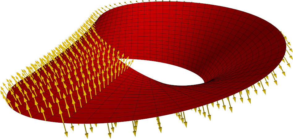
While already the initial announcement of Algosim 3.1 showed how to plot a surface in the form of a function graph, this example illustrates plotting a parameterised surface (as well as a vector field on a surface).
First, we need a parameterisation of the Möbius strip; we call this F. Also, for bonus points, we introduce a mapping NF that takes a surface parameterisation function, like our F, and returns its normal vector field. Using this mapping, the normal vector field of the Möbius strip is simply N ≔ NF(F). (This is a great example of the beauty of having functions as first-class objects.)
Here is the full code implementing this:
NF ≔ F ↦ ((u, v) ↦ normalized(diff(F(u, v), u, u) × diff(F(u, v), v, v)));

S ≔ ClearScene("Möbius strip");
AdjustVisual(S.axes, "visible": false);
AdjustVisual(S.view, "rθφ": ❨2.792, 72°, 20°❩);

F ≔ (u, v) ↦ ❨(1 + .5⋅v⋅cos(u/2))⋅cos(u), (1 + .5⋅v⋅cos(u/2))⋅sin(u), .5⋅v⋅sin(u/2)❩;
M ≔ surf([0, 2⋅π] × [−1, 1] @ F);
AdjustVisual(M,
  "show parameter curves": true,
  "parameter curve counts": ❨64, 16❩,
  "line width": .75,
  "unisided": true);

N ≔ NF(F);
VF ≔ VectorField([0, 2⋅π, π/32] × [−1, 1, 1/8] @ ((u, v) ↦ F(u, v) ~ N(u, v)));
AdjustVisual(VF,
  "size": 0.1,
  "anchor point": 1.03,
  "color": "gold")