Artiklar

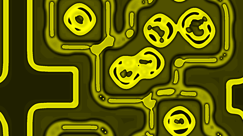
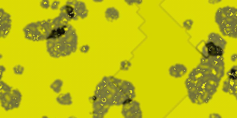
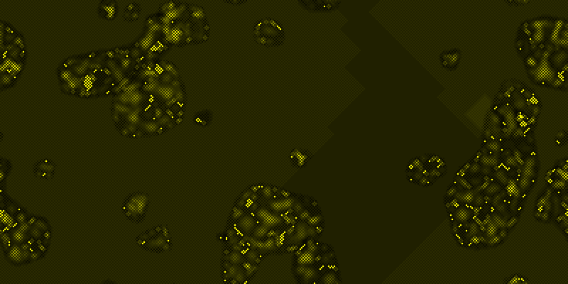
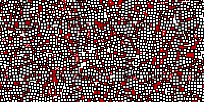
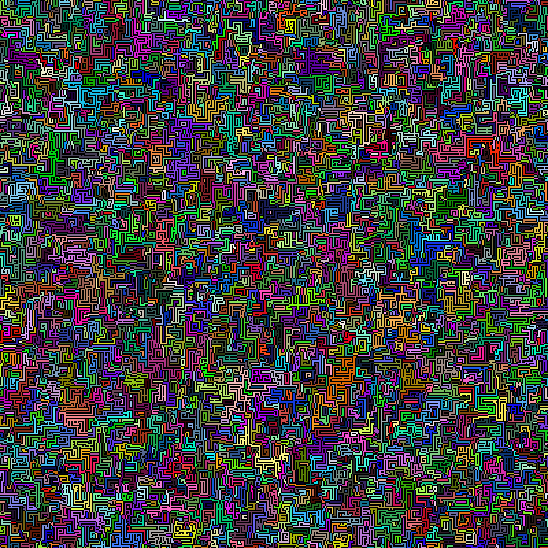
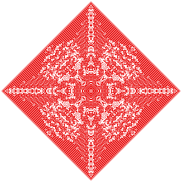
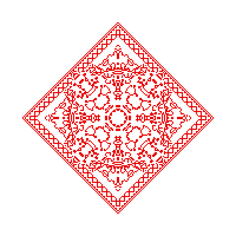
A new view of the automaton from yesterday:

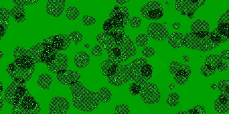
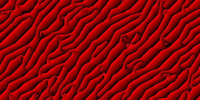
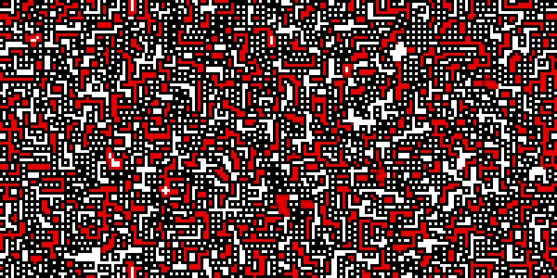
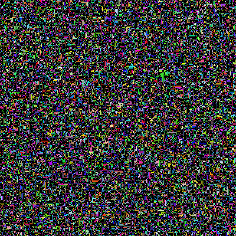
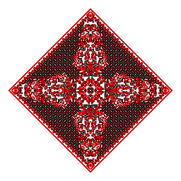
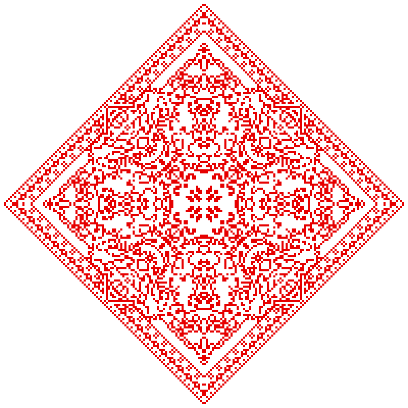
A second example of a simple coloured extended-range cellular automaton:

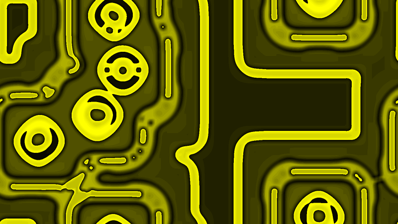
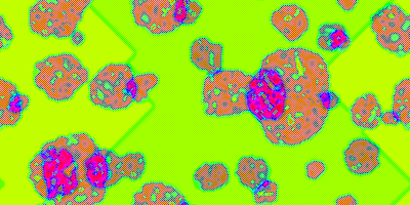
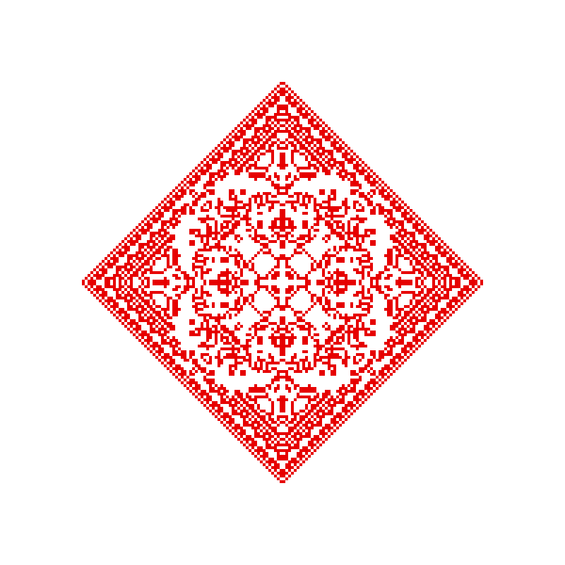
I have experimented a bit with coloured (RGB) extended-range cellular automata. Mathematically, these are ordinary N-state extended-range automata in which N = 256³, the values are interpreted as RGB colour codes and the rendering procedure uses the colour of the cell directly, instead of applying some arbitrary colour scheme. Below is a simple example I produced yesterday:

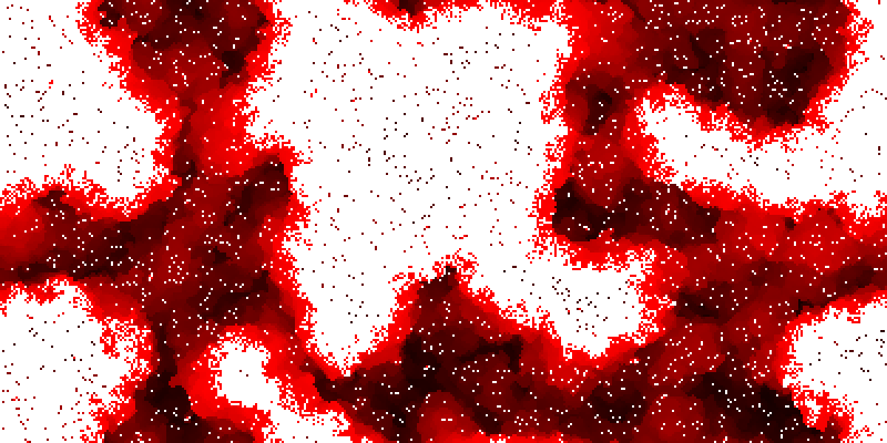
Today I give my first example of an extended-range cellular automaton. It is an N-state range-r automaton defined by the following rule: the new value of the cell is equal to the average of the values in the range-r Moore neighbourhood (including the cell itself) plus a constant increment. Typically I use N = 10, r = 32 or 36, and an increment of 10. Starting from random noise, this produces a small number of discrete circles (enclosed by squares) that evolve and expand until the entire region is filled with a chaotic mess. The most interesting images are obtained in the middle of this process. The following images shows generation 43:

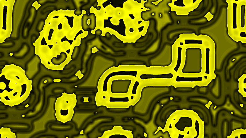
Another example (different simulation, same generation):

A bit later, the circles get rough boundaries:

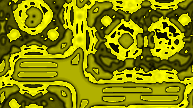
Another example:

All cellular automata I have considered this far have used the standard Moore neighbourhood, a 3×3 square with the current cell in the middle and eight neighbours. Yesterday I extended my program to support larger neighbourhoods. Now it supports neighbourhoods of arbitrary range. If the range is r, the neighbourhood consists of all cells you can reach in no more than r steps from the current cell, each step being horizontal, vertical, or diagonal. Hence, the range-r Moore neighbourhood is a square consisting of (2r + 1)² cells, with the current cell in the middle. r = 1 yields the standard eight-cell Moore neighbourhood.

The number of possible extended-range cellular automata is nearly ungraspable. Let us do some simple math.

• The number of life-like cellular automata in standard Moore neighbourhood is only 2¹⁸ = 262144, and I have investigated 2¹⁶ = 65536 of these individually (although extremely superficially).

• The number of binary cellular automata in standard Moore neighbourhood is 2²⁹ ≈ 1.34⋅10¹⁵⁴.

• The number of N-state cellular automata in standard Moore neighbourhood is N^N9. For N = 3, this yields approximately 1.51⋅10⁹³⁹¹; you can imagine what happens for N = 24...

• The number of life-like cellular automata with range r (that is, the binary automata that cares only about the cell itself and the number of living neighbours) is 2^2(2r + 1)2; for r = 2 and 3, this is equal to 1.13⋅10¹⁵ and 3.17⋅10²⁹, respectively.

• The number of binary range-r automata is 2^2(2r + 1)2. For r = 2, this is about 3.31⋅10^10100890. Imagine what happens for r = 3 and beyond.

• The number of N-state range-r cellular automata is N^N(2r + 1)2. Already N = 3 and r = 2 yields 1.32⋅10^404259404447.

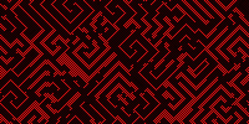
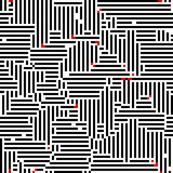
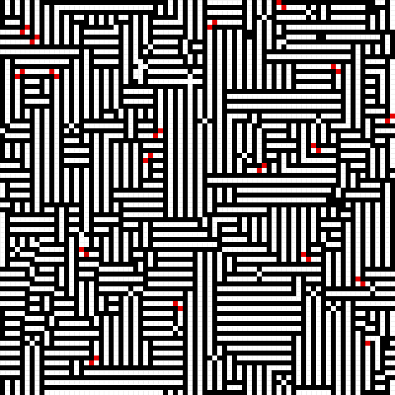
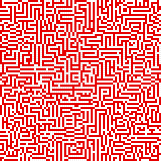
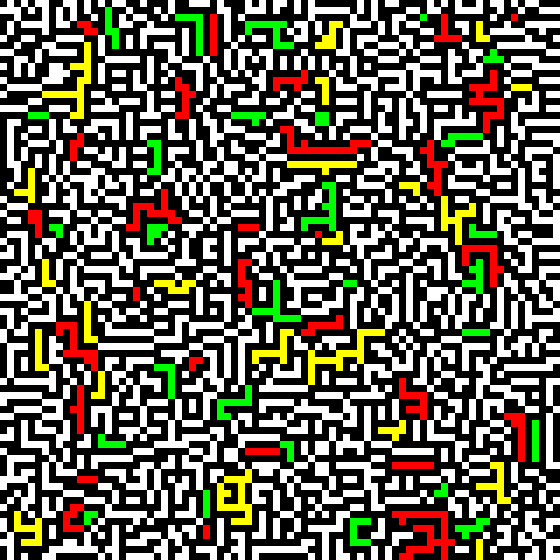
Recall “Rain” and “Inferno”, two cellular automata almost defined by the same rule; they only differ in the choice of the parameter θ, which is θ = N/24 for “Rain” and θ = N/12 for “Inferno”. If we let θ = −N/12, we obtain a new cellular automaton, which I call “Floor plan”. In general, this rule creates period-18 “floor plans”. A single such floor plan (for N = 24) is shown below:

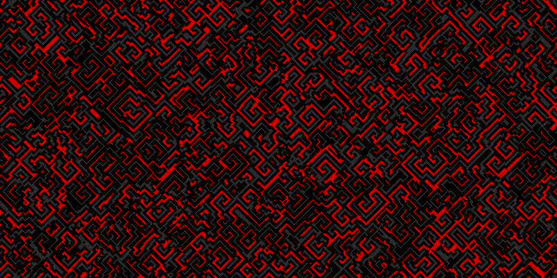
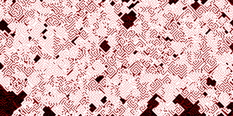
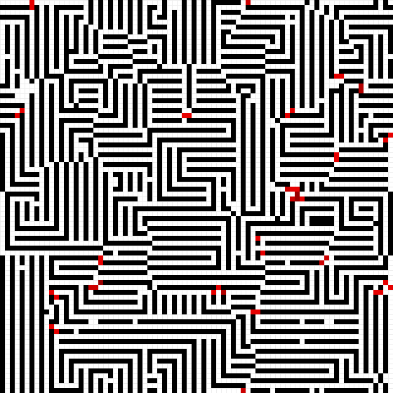
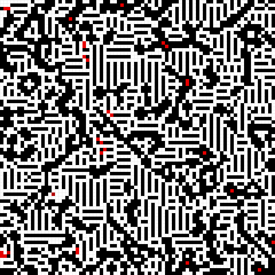
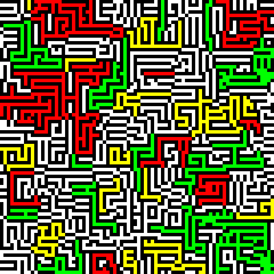
Although the image appears to be two-colour, it actually isn’t. By posterizing it to two colours, however, a true maze is obtained. And as far as mazes are concerned, this is a pretty nice one. Below a larger maze is shown and its main connected component is highlighted:

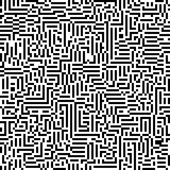
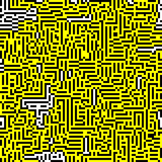
Today I present a particularly simple N-state cellular automaton. It is defined by the following rule: if a cell has two (or more) Moore neighbours with the same value as the cell itself, then the value of the cell is increased by one (mod N); otherwise, it is left unchanged. In this case, it is easy to see what kind of pattern is created simply by thinking about the rule. To confirm, here is a computer simulation showing a still image from the final stage (N = 96):

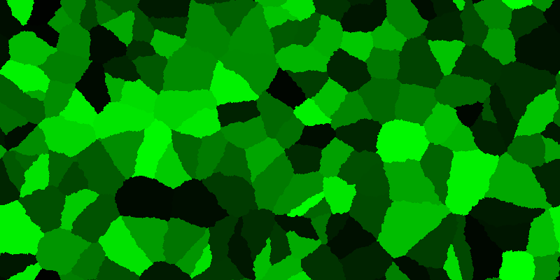
It is also easy to figure out what happens if N is changed; I leave this as an exercise to the reader.

Today we give another simple but visually pleasing example of an N-state CA: if the value of the cell is greater than the average of the von Neumann neighbours minus θ, decrease the value of the cell by one (mod N); otherwise, set it to the successor (mod N) of this average. N = 24 and θ = N/24 gives “Rain”, preferably rendered in shades of blue:

If instead θ = N/12, we obtain “Inferno”, preferably rendered in shades of red (or not at all).

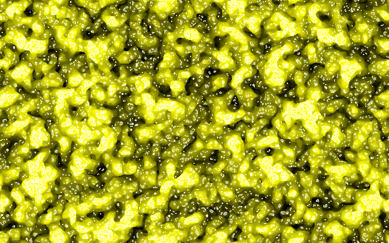
Both “Fuzz with dust” and “Dunes” contain the following rule as “subrules”: replace a cell’s value by the successor (mod N) of the average of the values of the von Neumann neighbours. How does this rule look on its own?

The answer is that it produces growing fluorescent cells on a folder-containing background:

The fluorescence becomes apparent when the background darkens, as it does cyclically:

A less zoomed-in picture (with a different colour scheme):

With the “Rainbow” colour scheme, the illusion of fluorescence disappears, but the images are still very pleasant:

A few weeks ago, I considered the following N-state cellular automaton rule: if the top-left neighbour of a cell has a value greater than N/2, then the value of the cell is increased by one (mod N); otherwise, the value is set to the successor of the average of the values of the von Neumann neighbours (mod N). The result looks like this (for N = 24):

Superficially, the image looks like dunes, but if you look more carefully, it might actually bear a stronger resemblance to a network of anastomosing capillaries. Experiments performed on small(er) grids (strongly) suggest that, in most cases, the grid eventually becomes filled with non-anastomosing, parallel vessels with periodically animated colours, the period being at least as big as the smallest dimension of the grid (often with equality, but sometimes equal to the other dimension, or much, much larger than any of those).

Multi-state cellular automata can be used to create intriguing visual effects. Today and the next few days I will give examples of such visuals. I start with an automaton I discovered yesterday, defined by the following rule: if the top-left neighbour has a value greater than the bottom-right neighbour, decrease the value of the cell (mod N); otherwise, set the cell’s value to the successor (mod N) of the average of the values of the von Neumann neighbours. This produces the following result (with N = 24):

I call it “Fuzz with dust”.

In addition to the generalisations to the standard cyclic cellular automaton we saw yesterday, it is natural to investigate what happens if you increase a cell’s value not by one, but by two, three, or more every time it should be updated (not altering the condition). It turns out, at least for N = 24 states and the standard threshold (1), that you obtain rounded square spirals if you increase by two instead of by one:

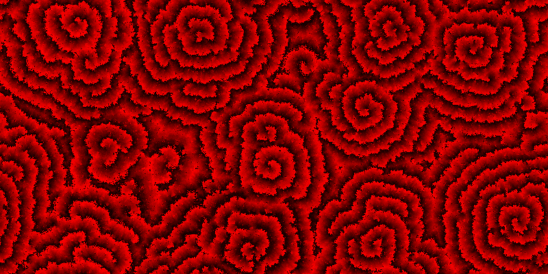
If you increase the increment to three, you make roses:

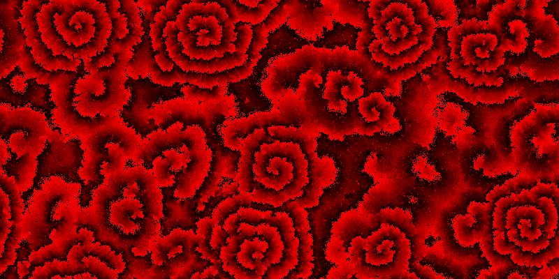
Eventually the roses cover the entire region:

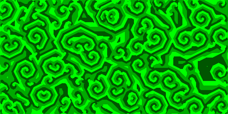
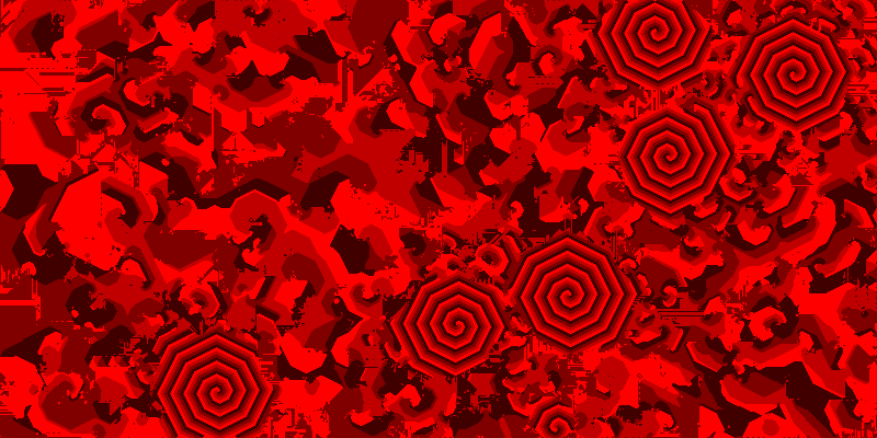
It is possible to alter the parameters of the cyclic cellular automaton. Obviously, the number of states N per cell can be varied. But it is also possible to change the “threshold”, defined as the number of neighbours with value n + 1 (mod N) needed for a cell to advance from n to n + 1 (mod N). Some of these variants have specific names, and two particularly neat ones are “313” (three states, threshold 3) and “Perfect” (four states, threshold 3), shown below.

The “313” rule creates a pattern of “moustaches”:

The “Perfect” rule creates octagonal spirals:

Tomorrow I will make a different kind of adjustment to the cyclic CA.

A well-known (non-life-like) cellular automaton is the cyclic automaton. In this system, each cell in a rectangular grid with toroidal topology is assigned any of N discrete values, ranging from 0 to N − 1. In each step, a cell with value n is assigned value n + 1 (mod N) if any (Moore) neighbour has this value; if no neighbour has value n + 1 (mod N), the cell is left unchanged.

I ran the simulation with N = 24 from an initial soup (in which every cell was randomly assigned any of the N values with equal probability). After about 400 generations, a period-24 stage is reached, where the entire plane consists of animated square spirals:

You may also have a look at the transformation from the initial soup to the final state. (Warning: somewhat awesome.)

According to both Wikipedia and mirekw.com, the cyclic ceullar automaton and its variants were first described by David Griffeath.

Today I give a first example of a non-life-like cellular automaton. It is a very similar beast, though: it still uses a rectangular grid with the toroidal topology, two possible states per cell, and the Moore neighbourhood, and the new state of a cell still is a function of the current states of the cell and its neighbours. However, in this automaton, it is not sufficient to know only the number of living neighbours to determine the new state of a cell.

To be specific, this automaton is very similar to B2/S23, but a dead cell comes to life iff it has precisely two live von Neumann neighbours; the survival condition still uses the Moore neighbourhood. Hence, in a sense, this automaton mixes the von Neumann and Moore neighbourhoods. Technically, though, it uses the entire Moore neighbourhood, but the birth condition cares about which neighbours are alive.

Below the ashes of this automaton (formed from a 50% random soup) is shown. It does produce a number of neat period-2, period-3, and period-4 oscillators.

Tomorrow I will give a much more interesting example of a non-life-like automaton.

Although I could probably spend a few more years discussing the properties of life-like cellular automaton rules, I feel it is time to end the introductory series. I do so by giving an example of a shrinking black blob in the Day and Night automaton (B3678/S34678).

However, you need not panic: by putting the life-like cellular automata aside for now, I can spend time investigating other types of automata.

Today we consider the final patterns (or ash) created by Game of Life itself (B3/S23). After trying a few times, I managed to produce a random initial 50% soup creating an ash containing instances of all of the three most common oscillators:

The final stage contains 71 blinkers (including ten traffic lights), two toads, and one beacon; these are the most common oscillators found in B3/S23 ash, in this order. As still lifes are concerned, we obtained 78 blocks, 47 beehives (including three honey farms), 17 loafs (but no bakery), seven boats, one tub, two ponds, and two ships (but no fleet).

After trying many more initial soups, I also managed to find one producing a pulsar in the end. The pulsar is the fourth most common oscillator.

This ash contains 96 blinkers (including eight traffic lights), one toad, no beacons, and one pulsar. The still lifes obtained were 98 blocks, 45 beehives (including one honey farm), 15 loafs (but no bakery), 13 boats, two tubs, three ponds, no ships (so obviously no fleet), and one barge.

Today, we continue to investigate the final or near-final stages of various life-like cellular automata. We begin with B5678/S023456 which represents a “class” of rules creating patterns that resemble lung tissue:

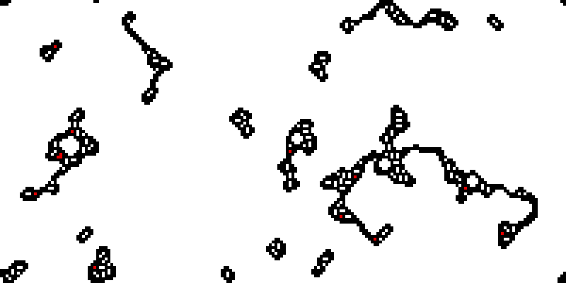
Many rules create ashes consisting of small black (stationary) objects. One example, B578/S024567, creates (microscopic) “worms” and debris:

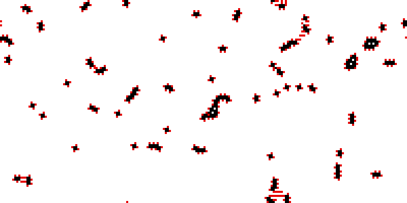
B568/S4567 creates other kinds of microscopic creatures, but no debris:

B4567/S567 creates opsonized bacteria:

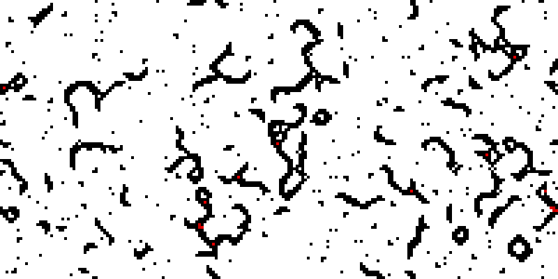
B378/S01235678 creates small islands of maze-like structures on a black background:

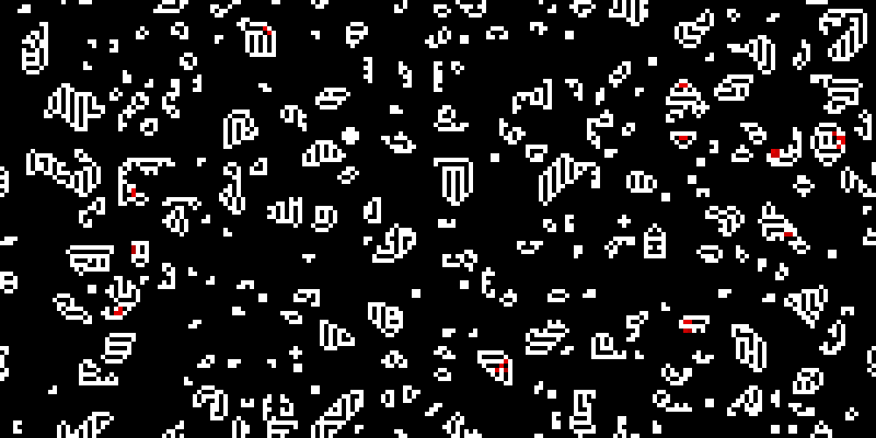
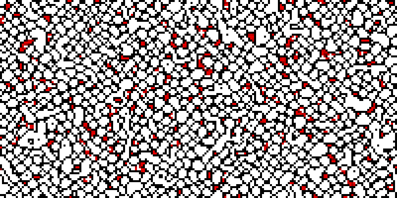
Finally, B278/S1456780 creates white lakes with red fish on a black background:

There are many life-like cellular automaton rules. To be specific, there are 262 144 of them. I have studied the rules that do not contain B0 or B1 in some detail. For each of these rules, I created an 80×80 torus with an initial 50% random soup and computed the 500th generation. In the obtained bitmap image, live cells were coloured according to their age (1: red; 2: a bit darker red; ...; 10 and beyond: black). Then I studied these 65536 images one screen (198 bitmaps) at a time, investigating many of them further.

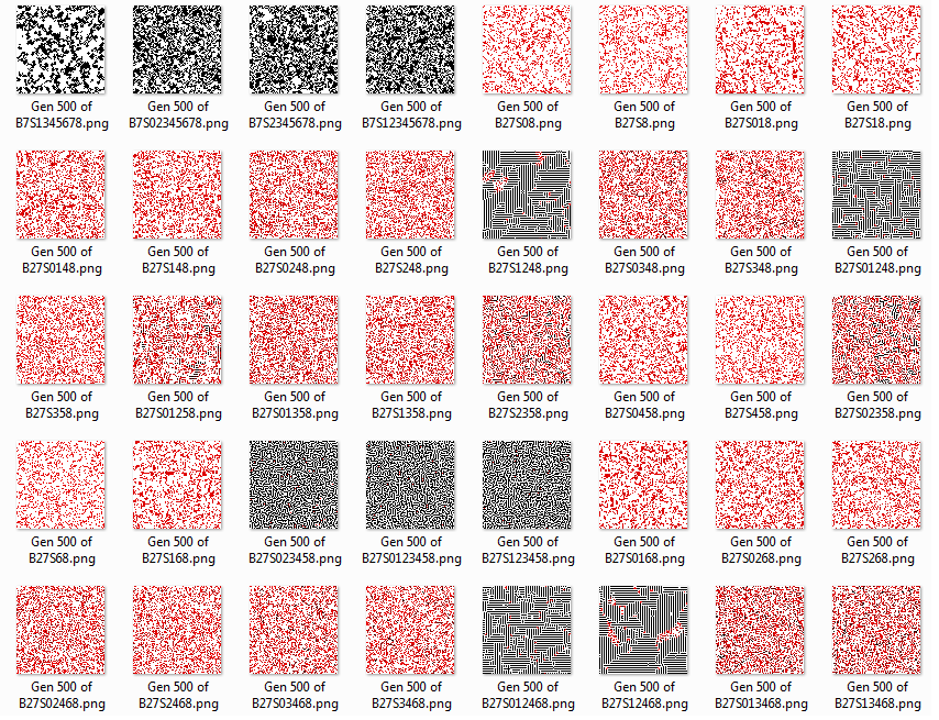
Not surprisingly, these 65536 bitmaps can very roughly be classified into a reasonably small number of “classes” according to the large-scale patterns they display. Two of these classes, the black and the red mazes, have already been described. Today we give a few other examples. Before doing so, however, three important points regarding the experiment should be made. First, some of the bitmaps didn’t represent the final stage of the simulation. Second, I did not obtain any information about the behaviour of the rules prior to the 500th generation (and sometimes the journey is more interesting than the final outcome). Third, many features of life-like rules cannot at all be discovered by an experiment like this. For instance, there are other seeds than the 50% random soup (like 2×2 squares and benzene rings) and spaceships aren’t detected. Still, the experiment gave me a better understanding of the life-like CA “zoo”.

A huge number of bitmaps display ongoing, chaotic activity with no “interesting” patterns; these bitmaps look rather similar to the initial soup (and the animations to noise), but with a slightly different distribution of live cells. In some cases, however, you clearly see some “interaction” between cells (B234/S023):

A very common type of pattern consists of red, black, and white pixels that form distinct patterns, typically with white rectangles with black borders surrounded by white and red areas. Below three such rules are shown:

B234567/S0234567:

B234678/S01234567:

B2345678/S01234567:

The last image doesn’t represent the final stage, which consists of only the red rectangle-like regions:

B234678/S7 belongs to a completely different “class”, in which two red “brush patterns” coexist on a white background:

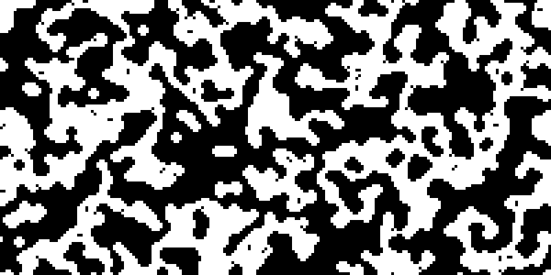
A huge number of rules create mainly (or, sometimes, entirely) black patterns, that is, stationary patterns, sometimes with oscillators, ranging from a number of small black objects on a white background to a bitmap almost entirely black. In between, sometimes large, irregular regions of (mainly) black and (mainly) white cells form; often boundaries between such regions oscillate in some way. A nice, (almost entirely) non-oscillating pattern with a black/white ratio close to 0.5 is formed quickly by B5678/S145678:

Tomorrow I will give six more examples (unless Linköping University contacts me, in which case I might suffer a breakdown).

The last two days we have become familiar with some of the CA maze-generating rules: “Maze” (B3/S12345), “Mazectric” (B3/S1234) and the B2(7)(8)/S(0)123(5)(6)(7)(8) family of very nice mazes. As noted, however, there are many more maze-generating rules, producing mazes with a number of different qualities. Today we will show a few more examples.

Some mazes are composed mainly (or even exclusively) of horizontal and vertical walls without corners, often found clustered together. For example, this is B2/S124, which consists of a single connected component:

The following maze (B3/S012358) is almost as simple, but also contains a few corners. As the reader can check for herself (e.g., using Win+R, pbrush, Enter), this one consists of one huge connected component and a few smaller components:

At the other extreme, this maze (B25/S23457) consists of a large number of (mostly either horizontal or vertical) small corridors not connected to each other:

Occasionally, you find a rule that forms voids (white-coloured areas) or rocks (black-coloured areas) in a maze (B278/S0124567):

There are also rules that produce mazes with very short walls, like B26/S012357:

Some mazes have additional features, like “force fields” (B23/S234):

A well-known example is “Maze with Mice” (B37/S12345):

Try also B2378/S1234.

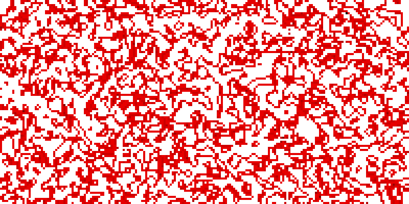
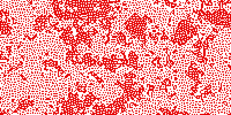
All mazes we have considered thus far have been almost stationary patterns (with the occasional oscillating corner, “force field”, or “mouse”), but there are also rules that form mazes that alternate between generations. Typically, a maze is replaced by its inverse in the next generation. I use the term “red mazes” to denote these, since they are shown in red in my software (because the walls consist of newly born cells in each generation). Below is B24567/S, one of these “red maze” rules:

In this article and the previous ones, we have only seen a small number of the many maze-forming rules. However, most of the remaining rules are close variants of the ones we have seen.

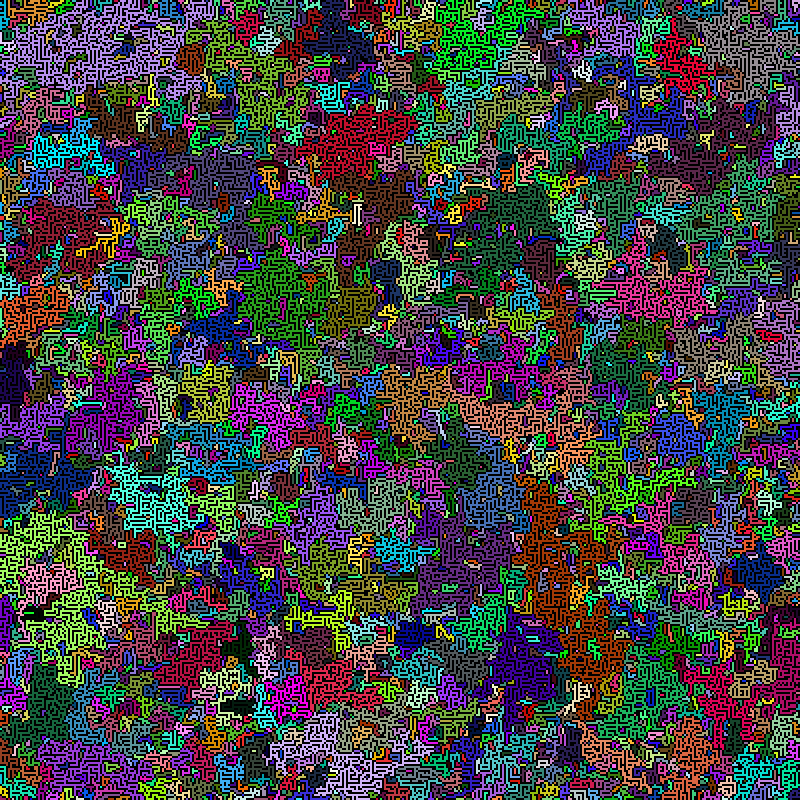
Let us continue yesterday’s discussion on maze-generating rules by considering some larger examples. By giving each connected component of “Maze” (B3/S12345) a unique colour, it is easy to see just how disconnected the maze is:

Applying the same processing to “Mazectric” (B3/S1234) we see that this maze is marginally better, but it is still highly disconnected:

As noted yesterday, we get a significant improvement by considering the inverse colouring of “Maze” (that is, by interpreting the white cells as walls and the black cells as corridors):

This makes the connected components a lot larger, but there is still quite a few of them. My proposed B2/S123, however, consists of one huge connected component and a fairly small number of very small or tiny components:

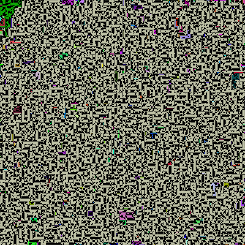
That’s what I call a maze!

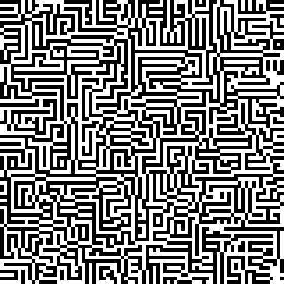
Among the 262144 possible life-like cellular automaton rules, quite a few generate mazes of various kinds. Among these, two are particularly well-known and are even named: “Maze” (B3/S12345) and “Mazectric” (B3/S1234). From an initial soup, these quickly make stationary mazes with the occasional oscillating corner (not shown below):

Maze:

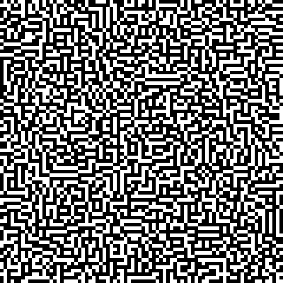
Mazectric:

I do not know why these two have been selected from the large number of maze-generating rules. In fact, I do not even consider them to be good examples of such rules, because the corridors they make are highly disconnected. This can be seen by trying a few flood-filling operations on the bitmaps:

Maze:

Mazectric:

Clearly, given two arbitrary points A and B in such a maze, it is highly unlikely that there is a path from A to B. (It appears like the situation gets better in the B3/S12345 (“Maze”) case if you reinterpret the white cells as the walls, but not very much.)

There are life-like maze-generating rules that create much better mazes in this regard, such as the B2(7)(8)/S(0)123(5)(6)(7)(8) rules. Below B2/S123 is shown:

B2/S123:

Trying a single flood-fill operation shows that this maze is much nicer (unless you are unlucky):

B2/S123:

Yesterday, we used the “Diamoeba” cellular automaton to give an example of CA dynamics. In that example, the boundary between a “diamond” of live cells and the surrounding dead cells fluctuated chaotically. A different boundary behaviour is exemplified by the rule B356/S014678, in which a random soup quickly will produce a large (possibly disconnected) region of mostly living cells surrounded by mostly dead cells (and a large number of small still-lifes and the occasional oscillator). The boundary of the large region is “burning”, and the total size of the region varies slowly with time:

A video is available (MP4, 36.3 MB) showing the first 3800 generations. If this particular simulation is allowed to proceed, the living pixels will win the battle. Indeed, just before generation 15000, the entire space consists of the region of living cells.

The “Diamoeba” cellular automaton (B35678/S5678) is a well-known life-like cellular automaton. Perhaps its most intriguing feature is the boundary fluctuation found on the “diamonds” formed by the automaton:

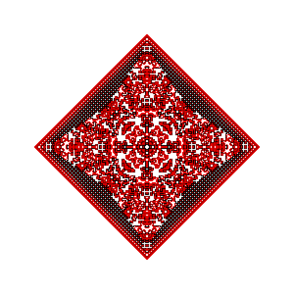
A few days ago we saw some of the patterns obtained from a 2×2 square using the “Persian rugs” (or “Serviettes”) cellular automaton (B234/S). Today we give a few other examples of “rugs” obtained using other rules.

Generation 135 of B234567/S124567:

Generation 146 of B234678/S8:

Generation 114 of B235678/S1234567:

Generation 101 of B2345678/S0238:

Yesterday, I investigated the life-like cellular automaton B268/S04567. This is an automaton in which most patterns explode, although a few still-lifes and oscillators exist. A random soup will, after a large number of generations, produce a black (stationary) pattern of small, irregular cells with common boundaries that fill the entire space. Some of these cells oscillate. This rule also supports a simple four-cell period-1 orthogonal spaceship travelling at the speed of light. Below two such ships collide, creating an explosion:

Somewhere at generation 2500, a periodic state, as described above, is reached. This state has period 1260, and looks roughly like this:

The life-like cellular automaton B234/S is known as “Persian rugs” or “Serviettes” because of the beautiful patterns it creates when the initial seed is a small, symmetric figure. Below, this automaton is run for 99 generations on a 200×200 grid with a central 2×2 square as the initial state. A family of lovely carpets of increasing size is obtained.

Among these patterns, some personal favourites are the following:

Generation 70:

Generation 73:

Generation 80:

Generation 97:

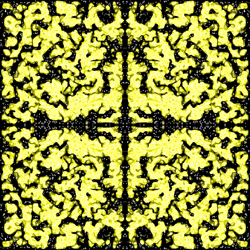
The life-like cellular automaton B378/S235678 is known as “Coagulations”. This automaton creates rather visually pleasing patterns. Below the simulation has been run for a few hundred generations on a 800×500 square grid with the torus topology and a 50 % soup as the initial state. The live cells are coloured according to their age (the number of generations they have been alive), from yellow (new live cell) to black (a few hundred generations old):

If the initial soup is symmetric, the state will be symmetric for all future generations:

To get a feeling for the dynamics of this CA, you may want to view an animation of the simulation from an initial soup or an initial small, central pattern. In these animations, only the first ten generations of a live cell are coloured.

Since Conway’s original Game of Life is the rule B3/S23, it is only appropriate that B3/S012345678 is named “Life without Death”. The following is a simulation of this cellular automaton on a 400×400 square grid with the topology of the plane (not torus) and an initial, small, random mass of pixels as the centre.

Besides the main, irregular, growth, a number of thin, regular, purely horizontal or vertical growth patterns are seen; these are known as “ladders”.

An interesting life-like cellular automaton is B1357/S1357. Nicknamed “Replicator”, this automaton will produce an infinite number of copies of any small initial figure. Below, this rule is applied to a rasterised version of the capital Latin letter “A”:

The simulation is run for 96 iterations. At each multiple of 16, the state consists of a number of perfect copies of the initial letter. (At the remaining multiples of 8, the state consists of a mixture of perfect and distorted copies.) To confirm that this is indeed a general phenomenon (and not something that requires the precise shape of the letter “A”), let us redo the experiment using a (rasterisation of a) benzene ring as the initial figure:

(Of course, the “chemical formulae” formed, consisting of adjoined benzene rings, are not valid.)

I have used some of my recently overwhelming spare time to program a simple cellular automata simulator. It is a native Win32 application able to run simulations on a finite rectangular grid with the topology of the plane or a torus. The computation is run in its own thread, different from the GUI thread, and the application supports binary, multi-state, and RGB automata with the Moore neighbourhood. All life-like cellular automata are supported (and are entered in the GUI using strings like “B3/S23”), and it is easy to hard-code other CAs. The application comes with a library of life-like CAs as well as number of interesting cyclic multi-state cellular automata.

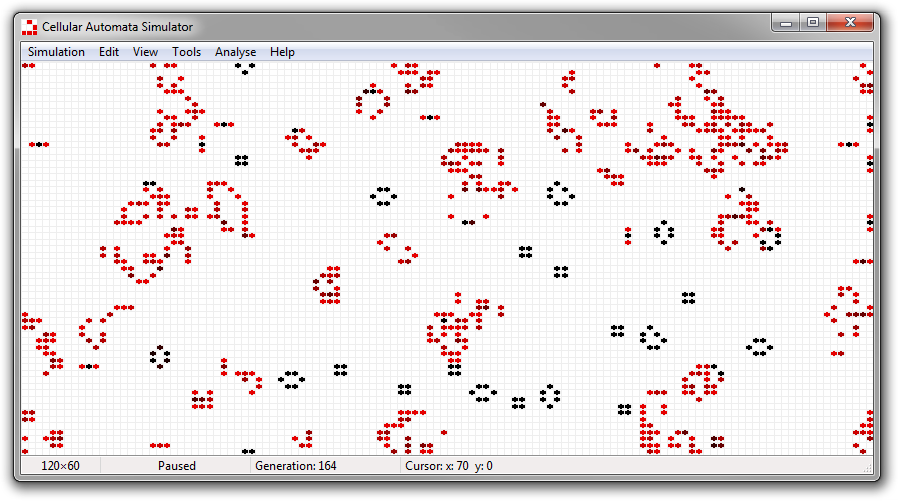
Below is a small Game of Life (B3/S23) simulation, starting from a random distribution of pixels on a 60×60 square grid with the torus topology. After 855 generations, a period-2 state is reached, containing a number of still lifes as well as eight blinkers (including one traffic light) and a toad.